Tutorial
Metal-organic framework MIL-53(Al) [3D material]
The stiffness matrix (coefficients in GPa) is input (Cij.dat)
Run: ElaTools.x
  > Select system dimension:
 =======================
  3D               => 3
  2D               => 2
 ========================
3
The compound is a 3D system, so we have to choose the number 3.
 > Select using output code:
============================================================
 IRelast-----------------------(       wein2k         )-=> 1
 Elast-------------------------(       wein2k         )-=> 2
 AELAS-------------------------(        VASP          )-=> 3
 ElaStic-----------------------(  QE,Wien2k,Exciting  )-=> 4
 Using Cij Tensor in Cij.dat---(     Other codes      )-=> 5
 Using EC Databank-------------(          MP          )-=> 6
============================================================
5
We use Cij.dat file. So we choose the number 5:
Initial output data:
#########################################################################

Cij:
      90.850000    20.410000    54.280000     0.000000     0.000000     0.000000
      20.410000    65.560000    12.360000     0.000000     0.000000     0.000000
      54.280000    12.360000    33.330000     0.000000     0.000000     0.000000
       0.000000     0.000000     0.000000     7.240000     0.000000     0.000000
       0.000000     0.000000     0.000000     0.000000    39.520000     0.000000
       0.000000     0.000000     0.000000     0.000000     0.000000     8.270000

Sij:
      0.4081110   -0.0018805   -0.6639371    0.0000000    0.0000000    0.0000000
     -0.0018805    0.0164084   -0.0030224    0.0000000    0.0000000    0.0000000
     -0.6639371   -0.0030224    1.1123872    0.0000000    0.0000000    0.0000000
      0.0000000    0.0000000    0.0000000    0.1381216    0.0000000    0.0000000
      0.0000000    0.0000000    0.0000000    0.0000000    0.0253036    0.0000000
      0.0000000    0.0000000    0.0000000    0.0000000    0.0000000    0.1209190

#########################################################################

==========================================================
 Elastic properties  |     Voigt     Reuss     Average
==========================================================
= Bulk modulus  (GPa)  |     40.427     5.019    22.723   =
= Shear modulus (GPa)  |     17.852     1.550     9.701   =
= Young modulus (GPa)  |     46.684     4.217    25.450   =
= P-wave modulus(GPa)  |    64.2293    7.0864   35.6579   =
= Poisson ratio        |     0.3075    0.4811    0.3943   = <--(  Ductile   regime      )
= Pugh ratio           |     2.2645    3.2379    2.3423   = <--(  Brittle   regime      )
==========================================================
> Universal anisotropy index (AU)        :   59.6328
> Log-Euclidean anisotropy parameter (AL):   13.1795
> Chung-Buessem Anisotropy Index (Ac)    :    0.8402
> Cauchy pressure(GPa) (Pc)              :    83.6100       <--(  Metallic-like bonding )
----------------------------------------------------------
This data is stored in the DATA.out file. We need another input to continue the EAlTools.x,
> Select the (m k l) index for 2D cut:
1 1 0
We select (1 1 0) palne
Then, the other output data listed in DATA.out file are as follows:
==================================================> Youngs Modulus
Max(GPa) Min(GPa)
94.71 0.90
------------------------------------------
Theta Phi Theta Phi
2.23 6.28 3.14 0.00
------------------------------------------
x y z x y z
0.79 -0.00 -0.61 0.00 0.00 -1.00
==================================================
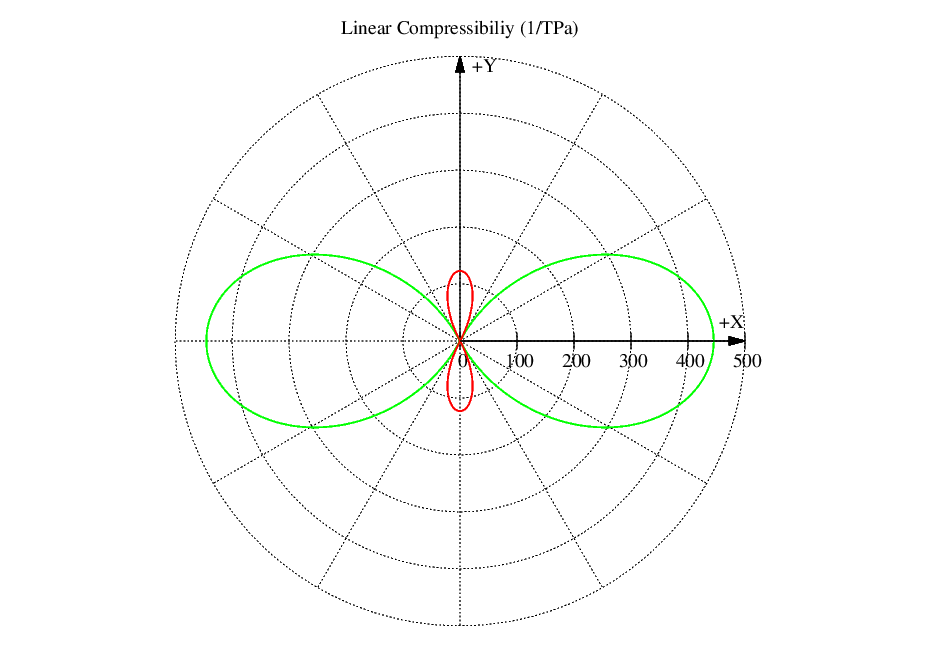
==================================================> Linear Compressibiliy
Max(TPa-1) Min(TPa-1)
445.428 -257.707
------------------------------------------
Theta Phi Theta Phi
3.14 0.00 1.57 6.28
------------------------------------------
x y z x y z
0.00 0.00 -1.00 1.00 -0.00 0.00
==================================================
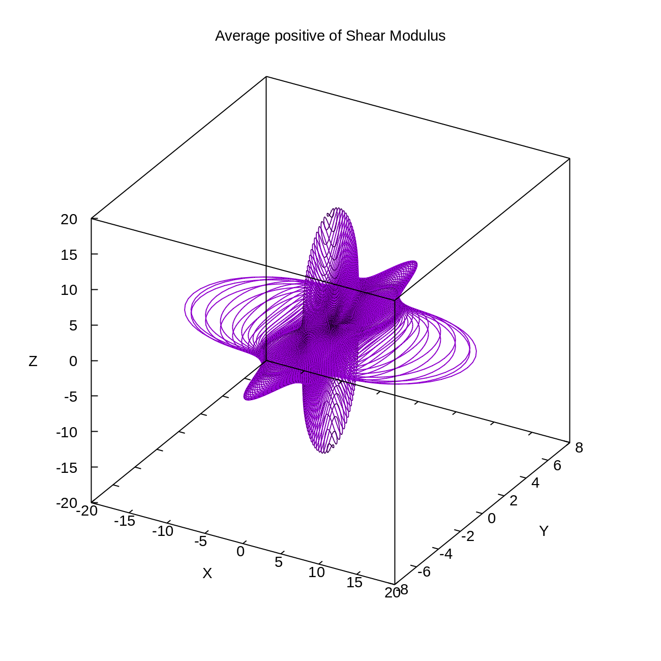
==================================================> Shear Modulus
Max(GPa) Min(GPa)
39.52 0.35
------------------------------------------
Theta Phi Theta Phi
3.14 0.00 2.36 6.28
------------------------------------------
x y z x y z
0.00 0.00 -1.00 0.71 -0.00 -0.71
==================================================
==================================================> Bulk Modulus
Max(GPa) Min(GPa)
3647.02 -95238.29
------------------------------------------
Theta Phi Theta Phi
1.85 2.01 0.93 6.13
------------------------------------------
x y z x y z
-0.41 0.87 -0.28 0.79 -0.13 0.60
==================================================
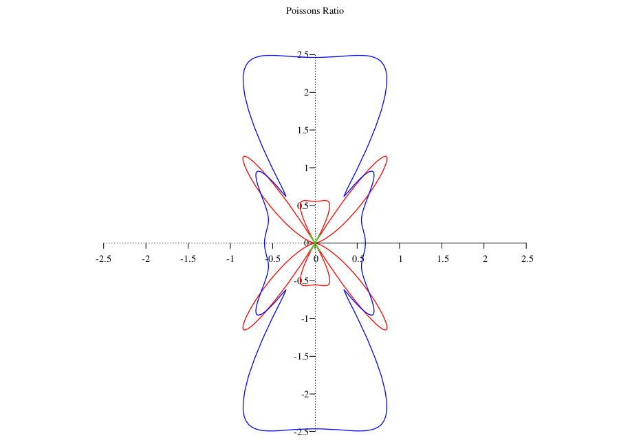
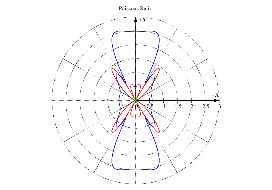
==================================================> Poissons Ratio
Max Min
2.977 -2.400
------------------------------------------
Theta Phi Theta Phi
1.57 4.21 1.92 4.71
------------------------------------------
x y z x y z
-0.48 -0.88 0.00 -0.00 -0.94 -0.34
==================================================
==================================================> Pugh Ratio
Max Min
3.22 -10.18
------------------------------------------
Theta Phi Theta Phi
3.14 0.00 1.57 6.28
------------------------------------------
x y z x y z
0.00 0.00 -1.00 1.00 -0.00 0.00
==================================================
==================================================> Sound
Transverse high Longitudinal Transverse low
49.82 33.33 0.35
==================================================
> NOTE :The above information is stored in 'DATA.out' file.
#==================================#
Note
Sound and Pugh Ratio are being tested!
In the following:
> Do you want to plot data? (Y/N):
If you select N, the name.dat files will be saved in the DataFile folder. If you select Y, the ploting process is activated and Figures are saved in the PicFils folder. We select Y: Some temporary Figs.:
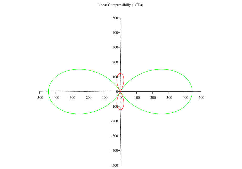


It is better to use dat2wrl_lapw, dat2gnu_lapw and dat2agr_lapw to draw more advanced 2d and 3D Figs.. For example, 3D representation of Linear Compressibiliy and Poissons Ratio by
$ dat2wrl_lapw com
$ dat2wrl_lapw poi
outpot files: Poissons.wrl and Compressibiliy.wrl, And using View3dscene , we will see it.


2D representation of Poisson’s ratio and Linear Compressibiliy in the (1 1 0 ) plane,
$ dat2gnu_lapw poi
> Using: go to gnuplot, call 'poissons.gpi' '0.2' '0.6' (or other scale)

$ dat2gnu_lapw com
> Using: go to gnuplot, call 'compressibiliy.gpi' '25' '120' (or other scale)
Resalt: poissons.ps and compressibiliy.ps
Gallium Thiophosphate-GaPS4 [2D material]
The stiffness matrix (coefficients in N/m) is input (Cij-2D.dat)
Run: EalTools.x
  > Select system dimension:
 =======================
  3D               => 3
  2D               => 2
 ========================
2
The compound is a 2D system, so we have to choose the number 2.
 > Select using output code:
==================================================
 Using Cij Tensor in Cij.dat   (other codes) => 3
==================================================
3
We use Cij-2D.dat file. So we choose the number 3:
Initial output data:
########################################

Cij:
   4.450000    3.630000    0.000000
   3.630000   19.220000    0.000000
   0.000000    0.000000    4.710000

Sij:
   0.265645   -0.050171    0.000000
  -0.050171    0.061505    0.000000
   0.000000    0.000000    0.212314

########################################
================================================
             Elastic properties
================================================
= Young modulus [Ex]  (N/m)     3.764          =
= Young modulus [Ey]  (N/m)    16.259          =
= Shaer modulus [Gxy] (N/m)     4.710          =
= Shaer modulus [Gv]  (N/m)     4.406          =
= Shaer modulus [Gr]  (N/m)     3.126          =
= Area modulus  [Kv]  (N/m)     7.732          =
= Area modulus  [Kr]  (N/m)     4.409          =
= Poisson ratio [vxy]           0.189          =
= Poisson ratio [vyx]           0.816          =
==================================================================
= Elastic anisotropy index (A_SU):                 0.579          =
= Ranganathan Elastic anisotropy index (A_SU):     1.573          =
= Kube Elastic anisotropy index (A_SU):            0.322          =
==================================================================
 > Preparing data. please wait...

==================================================> Youngs Modulus
 Maximum value of Youngs Modulus =     3.4599       Phi=   99.0000 degree
 MINimum value of Youngs Modulus =     0.7992       Phi=    0.0000 degree
==================================================

==================================================> Poissons Ratio
 Maximum value of Poissons Ratio =     0.6860       Phi=   90.0000 degree
 Minimum value of Poissons Ratio =    -0.0391       Phi=   46.8000 degree
==================================================>
In the following:
> Do you want to prepare the data for ploting? (Y/N):
If you select N, the name.dat files will be saved in the DataFile folder. If you select Y, the ploting process is activated and Figures are saved in the PicFils folder. We select Y:
resalts Figs.: 2D_sys_Poissons.ps and 2D_sys_Young.ps.


Using
$ dat2gnu_lapw D2
 > Using: go to gnuplot, call '2Dpoissons.gpi' '0.2' '0.6' (or other scale)
 > Using: go to gnuplot, call '2Dyoung.gpi' '50' '100' (or other scale)
, you can also draw better charts.


Gallium arsenide [3D material]
The stiffness matrix (coefficients in GPa) is input (Cij.dat)
Run: EalTools.x
  > Select system dimension:
 =======================
  3D               => 3
  2D               => 2
 ========================
3
The compound is a 3D system, so we have to choose the number 3.
 > Select using output code:
============================================================
 IRelast-----------------------(       wein2k         )-=> 1
 Elast-------------------------(       wein2k         )-=> 2
 AELAS-------------------------(        VASP          )-=> 3
 ElaStic-----------------------(  QE,Wien2k,Exciting  )-=> 4
 Using Cij Tensor in Cij.dat---(     Other codes      )-=> 5
 Using EC Databank-------------(          MP          )-=> 6
============================================================
5
We use Cij.dat file. So we choose the number 5.
> Want to calculate phase and group velocities? (Y/n)
Y
At this point we are going to calculate the phase and group velocities (add in >v.1.5 ), So, select Y.
Density of Compound (kg/m^3):
note: If you don't know, enter 0
Density of GaAs compound is 5307.0 kg/m^3. But if you do not know it, dens_lapw will calculate it for you. Just enter 0.
we enter 5307.0,therefore
  > Density of Compound =   5307.00000000000
#########################################################################
Cij:
    118.800000    53.800000    53.800000     0.000000     0.000000     0.000000
     53.800000   118.800000    53.800000     0.000000     0.000000     0.000000
     53.800000    53.800000   118.800000     0.000000     0.000000     0.000000
      0.000000     0.000000     0.000000    59.400000     0.000000     0.000000
      0.000000     0.000000     0.000000     0.000000    59.400000     0.000000
      0.000000     0.000000     0.000000     0.000000     0.000000    59.400000

Sij:
     0.0117287   -0.0036559   -0.0036559    0.0000000    0.0000000    0.0000000
    -0.0036559    0.0117287   -0.0036559    0.0000000    0.0000000    0.0000000
    -0.0036559   -0.0036559    0.0117287    0.0000000    0.0000000    0.0000000
     0.0000000    0.0000000    0.0000000    0.0168350    0.0000000    0.0000000
     0.0000000    0.0000000    0.0000000    0.0000000    0.0168350    0.0000000
     0.0000000    0.0000000    0.0000000    0.0000000    0.0000000    0.0168350

#########################################################################


==========================================================
 Elastic properties  |     Voigt     Reuss     Average
==========================================================
= Bulk modulus  (GPa)|     75.467    75.467    75.467   =
= Shear modulus (GPa)|     48.640    44.626    46.633   =
= Young modulus (GPa)|    120.114   111.833   115.974   =
= P-wave modulus(GPa)|   140.3200  134.9672  137.6436   =
= Poisson ratio      |     0.2347    0.2530    0.2439   = <--(  Brittle   regime      )
= Pugh ratio         |     1.5515    1.6911    1.6183   = <--(  Brittle   regime      )
==========================================================
> Universal anisotropy index (AU)        :    0.4498
> Log-Euclidean anisotropy parameter (AL):    0.4436
> Chung-Buessem Anisotropy Index (Ac)    :    0.0430
> Cauchy pressure(GPa) (Pc)              :    59.4000     <--(  Metallic-like bonding)
----------------------------------------------------------

> Output for  ( 1.0, 0.0, 0.0) plane

 =================================================> Youngs Modulus
  Max(GPa)             Min(GPa)          Anisotropy
  141.02                85.26               1.65
------------------------------------------
  Theta   Phi          Theta   Phi
  126.0  316.8         180.0    0.0
------------------------------------------
   x     y     z        x     y     z
  0.59 -0.55 -0.59     0.00  0.00 -1.00
==================================================

 ==================================================> Linear Compressibiliy
  Max(TPa-1)           Min(TPa-1)           Anisotropy
    4.417                 4.417              1.000
------------------------------------------
  Theta   Phi          Theta   Phi
 147.6 198.0            102.6  97.2
------------------------------------------
   x     y     z        x     y     z
 -0.51 -0.17 -0.84    -0.12  0.97 -0.22
==================================================

 ==================================================> Shear Modulus
  Max(GPa)             Min(GPa)           Anisotropy
   59.40                32.50               1.83
------------------------------------------
  Theta   Phi          Theta   Phi
 180.0   0.0            135.0 360.0
------------------------------------------
   x     y     z        x     y     z
  0.00  0.00 -1.00     0.71 -0.00 -0.71
==================================================

 ==================================================> Bulk Modulus
   Max(GPa/100)              Min(GPa/100)           Anisotropy
        2.26                    2.26               1.00
------------------------------------------
  Theta   Phi          Theta   Phi
 102.6  97.2            147.6 198.0
------------------------------------------
   x     y     z        x     y     z
 -0.12  0.97 -0.22    -0.51 -0.17 -0.84
==================================================

 ==================================================> Phase P-Mode
   Max(km/s)              Min(km/s)           Anisotropy
        5.40                    4.73               1.14
------------------------------------------
  Theta   Phi          Theta   Phi
  54.0 223.2            180.0   0.0
------------------------------------------
   x     y     z        x     y     z
  0.55  0.08 -0.83    -0.80  0.00 -0.60
==================================================

 ==================================================> Phase Fast-Mode
   Max(km/s)              Min(km/s)           Anisotropy
        3.35                    3.35               1.00
------------------------------------------
  Theta   Phi          Theta   Phi
 124.2 360.0            180.0   0.0
------------------------------------------
   x     y     z        x     y     z
  0.28 -0.95  0.11    -0.80  0.00 -0.60
==================================================

 ==================================================> Phase Slow-Mode
   Max(km/s)              Min(km/s)           Anisotropy
        3.35                    0.00                Inf
------------------------------------------
  Theta   Phi          Theta   Phi
 180.0   0.0            180.0   0.0
------------------------------------------
   x     y     z        x     y     z
 -0.80  0.00 -0.60    -0.80  0.00 -0.60
==================================================

 ==================================================> Group P-Mode
   Max(km/s)              Min(km/s)           Anisotropy
        5.40                    4.73               1.14
------------------------------------------
  Theta   Phi          Theta   Phi
  54.0 316.8            180.0   0.0
------------------------------------------
   x     y     z        x     y     z
  0.49 -0.27 -0.83    -0.80  0.00 -0.60
==================================================

 ==================================================> Group Fast-Mode
   Max(km/s)              Min(km/s)           Anisotropy
        3.37                    3.35               1.01
------------------------------------------
  Theta   Phi          Theta   Phi
  79.2 133.2            180.0   0.0
------------------------------------------
   x     y     z        x     y     z
 -0.19 -0.58 -0.79    -0.80  0.00 -0.60
==================================================

 ==================================================> Group Slow-Mode
   Max(km/s)              Min(km/s)           Anisotropy
        3.35                    3.35               1.00
------------------------------------------
  Theta   Phi          Theta   Phi
 180.0   0.0            180.0   0.0
------------------------------------------
   x     y     z        x     y     z
 -0.80  0.00 -0.60    -0.80  0.00 -0.60
==================================================

 ==================================================> Poisson's Ratio
     Max                  Min            Anisotropy
  0.443                0.021              21.21
------------------------------------------
  Theta   Phi          Theta   Phi
 135.0 360.0            135.0 360.0
------------------------------------------
   x     y     z        x     y     z
  0.71 -0.00 -0.71     0.71 -0.00 -0.71
==================================================
Finally, for example, we use the following command to visualize a 2D heat map of Poisson’s Ratio (Figure poissons_smap.png is the result.):
dat2gnu_lapw hmpoi
